

Trip Advisor: Boston, London or Dubai?
Introduction
There are generally two types of travelers: the spontaneous type and the researcher. The spontaneous type will usually book the flight and hotels without much second thought, whereas the researcher type will only start booking when they have read every guide and review out there. User-based reviews bring particular insight into a city’s attractions, hotels and restaurants since it provides recent, honest opinions from people who are in the same situation as you plan to be.
However, it turns out that when you are the researcher type, it can be overwhelming to go through so many reviews. There might be one negative review which will trump the hundreds of other positive reviews leaving you with a negative sentiment of the place. In reality however, we do not know the context of that review, and could be missing out on an amazing experience.
This report outlines an analysis of user reviews from TripAdvisor.com for three cities: Boston, Dubai and London. It aims to provide insights on people’s sentiment of their experience, differences between the three cities and what travel experience makes them unique.
Data Collection Methodology
The data used for this report has been scraped from TripAdvisor.com reviews page for each city. The reviews were collected without any form of identification of the user. Only the 100 most recent reviews for each city were collected.
For this specific process, I used Selector Gadget, an open source Google Chrome extension to scrape the website. To import it into R, I used the rvest package (Wickham, 2019) in addition to other necessary packages for this analysis:
# loading necessary packages
library(rvest)
library(dplyr)
library(stringr)
library(tidytext)
library(tidyverse)
library(tm)
library(tidyr)
library(scales)
library(reshape2)
library(wordcloud)
library(igraph)
library(ggraph)
In order to have a large enough amount of reviews, I decided to gather the 5 most recent review pages, each with 20 reviews (total 100 reviews per city). The following process was repeated for both Dubai and London:
# STEP 1: Data Scraping
# Top 5 Review Pages of Boston
b_url1         <- "https://www.tripadvisor.com/AllReviews-g60745"
b_html1        <- read_html(b_url1)
b_guide_html1  <- html_nodes(b_html1,'.partial_entry')
b_guide1       <- html_text(b_guide_html1)
b_df1          <- data_frame(line=1:20, text=b_guide1)
b_url2         <- "https://www.tripadvisor.com/AllReviews-g60745-or20-Boston_Massachusetts.html"
b_html2        <- read_html(b_url2)
b_guide_html2  <- html_nodes(b_html2,'.partial_entry')
b_guide2       <- html_text(b_guide_html2)
b_df2          <- data_frame(line=1:20, text=b_guide2)
b_url3         <- "https://www.tripadvisor.com/AllReviews-g60745-or40-Boston_Massachusetts.html"
b_html3        <- read_html(b_url3)
b_guide_html3  <- html_nodes(b_html3,'.partial_entry')
b_guide3       <- html_text(b_guide_html3)
b_df3          <- data_frame(line=1:20, text=b_guide3)
b_url4         <- "https://www.tripadvisor.com/AllReviews-g60745-or60-Boston_Massachusetts.html"
b_html4        <- read_html(b_url4)
b_guide_html4  <- html_nodes(b_html4,'.partial_entry')
b_guide4       <- html_text(b_guide_html4)
b_df4          <- data_frame(line=1:20, text=b_guide4)
b_url5         <- "https://www.tripadvisor.com/AllReviews-g60745-or80-Boston_Massachusetts.html"
b_html5        <- read_html(b_url5)
b_guide_html5  <- html_nodes(b_html5,'.partial_entry')
b_guide5       <- html_text(b_guide_html5)
b_df5          <- data_frame(line=1:20, text=b_guide5)

boston <- bind_rows(b_df1, b_df2, b_df3, b_df4, b_df5)
After import, each city’s reviews were a data frame with two variables: line and text. Line corresponds to the review number and text the content of the review. Data cleaning consisted of removing common words (stop words) and numbers. No typos were removed. Names of the cities were removed as to not skew results.
# STEP 2: Data Cleaning and Tokenization

## Custom Stop Words
custom_stop_words <- tribble(~word, ~lexicon,
                             "boston", "CUSTOM",
                             "dubai", "CUSTOM",
                             "london", "CUSTOM",
                             "5", "CUSTOM",
                             "2","CUSTOM",
                             "it’s","CUSTOM",
                             "15","CUSTOM",
                             "24","CUSTOM",
                             "1","CUSTOM",
                             "6","CUSTOM",
                             "8","CUSTOM",
                             "4","CUSTOM",
                             "10","CUSTOM",
                             "40","CUSTOM",
                             "12","CUSTOM",
                             "3","CUSTOM",
                             "30","CUSTOM",
                             "7","CUSTOM",
                             "i’ve","CUSTOM")
stop_words2 <- stop_words %>%
  bind_rows(custom_stop_words)

## Boston
boston_tokens <- boston %>%
  unnest_tokens(word, text) %>%
  anti_join(stop_words2)

## Dubai
dubai_tokens <- dubai %>%
  unnest_tokens(word, text) %>%
  anti_join(stop_words2)

## London
london_tokens <- london %>%
  unnest_tokens(word, text) %>%
  anti_join(stop_words2)
Analysis
Positive and Negative Sentiments
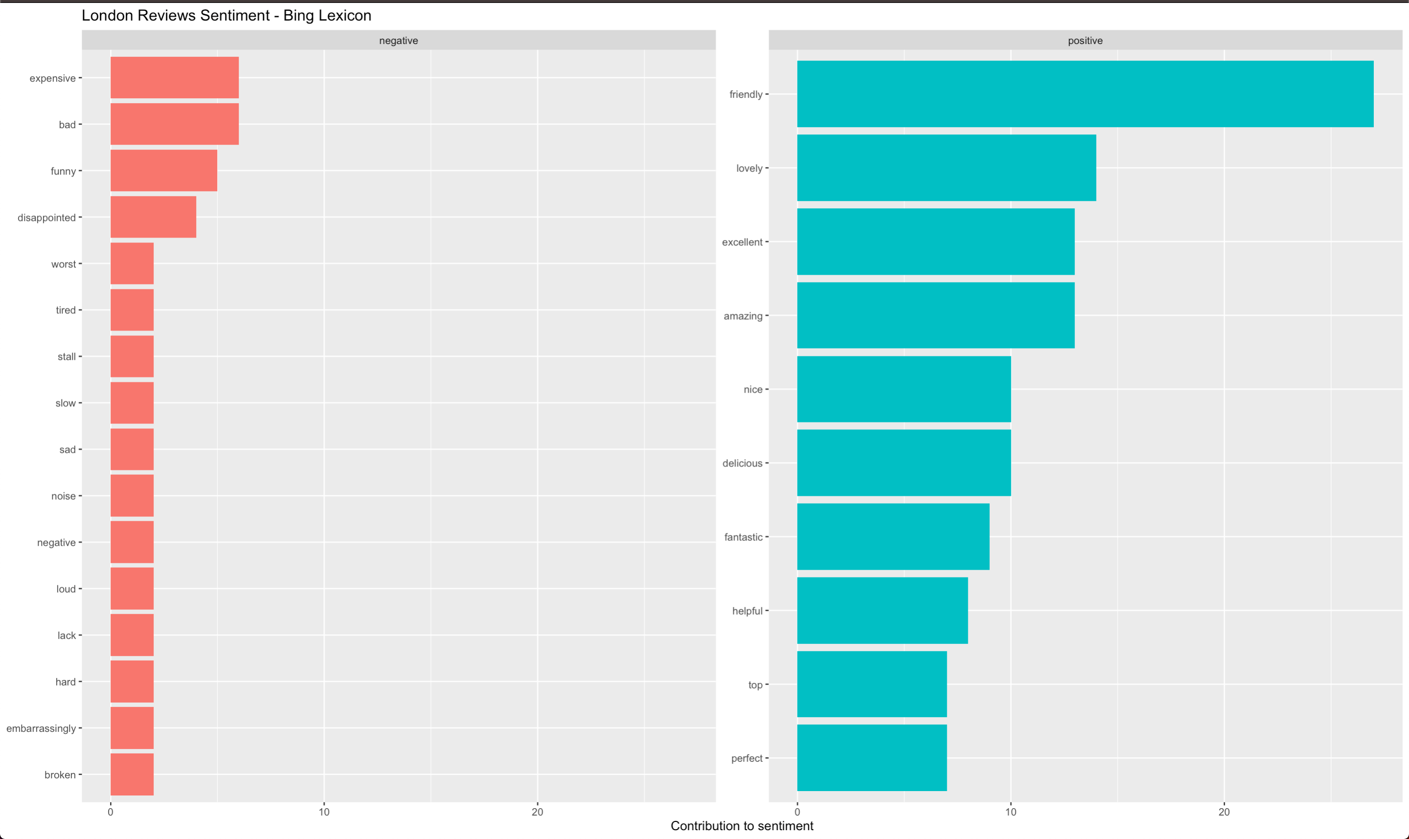
As mentioned, in social media reviews, the negative words tend to stick out amongst a sea of positive comments (Beaton, 2018). The analysis of reviews for Boston, Dubai and London shed a light on why that might be the case: common positive words used in reviews are very general in all cities, whereas negative words paint a very city-specific image to the reader.
# STEP 3: Frequency - Sentiment Analysis (Bing Lexicon)

## BOSTON
boston_bing <- boston_tokens %>%
  inner_join(get_sentiments("bing")) %>%
  count(word, sentiment, sort=T) %>%
  group_by(sentiment) %>%
  top_n(10, n) %>%
  ungroup() %>%
  mutate(word=reorder(word, n)) %>%
  ggplot(aes(word, n, fill=sentiment)) +
  geom_col(show.legend = FALSE) +
  facet_wrap(~sentiment, scales = "free_y")+
  labs(y="Contribution to sentiment", x=NULL, title = "Boston Reviews Sentiment - Bing Lexicon")+
  coord_flip()

## DUBAI
dubai_bing <- dubai_tokens %>%
  inner_join(get_sentiments("bing")) %>%
  count(word, sentiment, sort=T) %>%
  group_by(sentiment) %>%
  top_n(10, n) %>%
  ungroup() %>%
  mutate(word=reorder(word, n)) %>%
  ggplot(aes(word, n, fill=sentiment)) +
  geom_col(show.legend = FALSE) +
  facet_wrap(~sentiment, scales = "free_y")+
  labs(y="Contribution to sentiment", x=NULL, title = "Dubai Reviews Sentiment - Bing Lexicon")+
  coord_flip()

## LONDON
london_bing <- london_tokens %>%
  inner_join(get_sentiments("bing")) %>%
  count(word, sentiment, sort=T) %>%
  group_by(sentiment) %>%
  top_n(10, n) %>%
  ungroup() %>%
  mutate(word=reorder(word, n)) %>%
  ggplot(aes(word, n, fill=sentiment)) +
  geom_col(show.legend = FALSE) +
  facet_wrap(~sentiment, scales = "free_y")+
  labs(y="Contribution to sentiment", x=NULL, title = "London Reviews Sentiment - Bing Lexicon")+
  coord_flip()
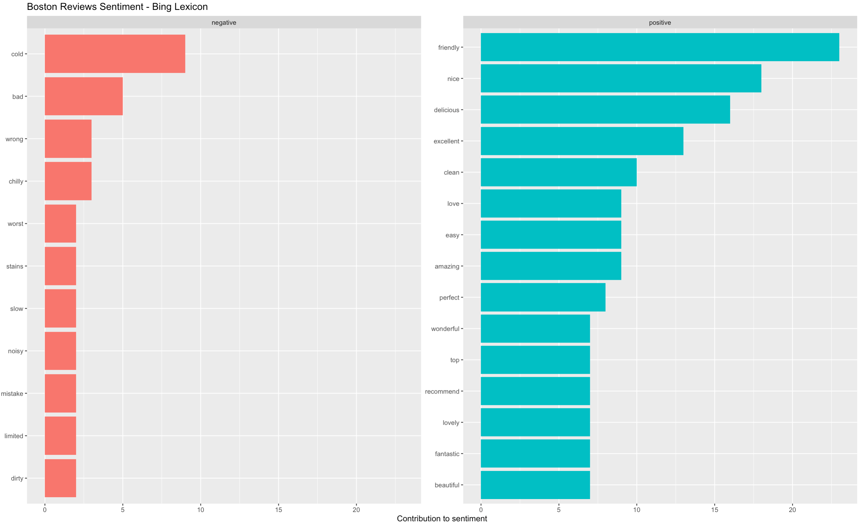
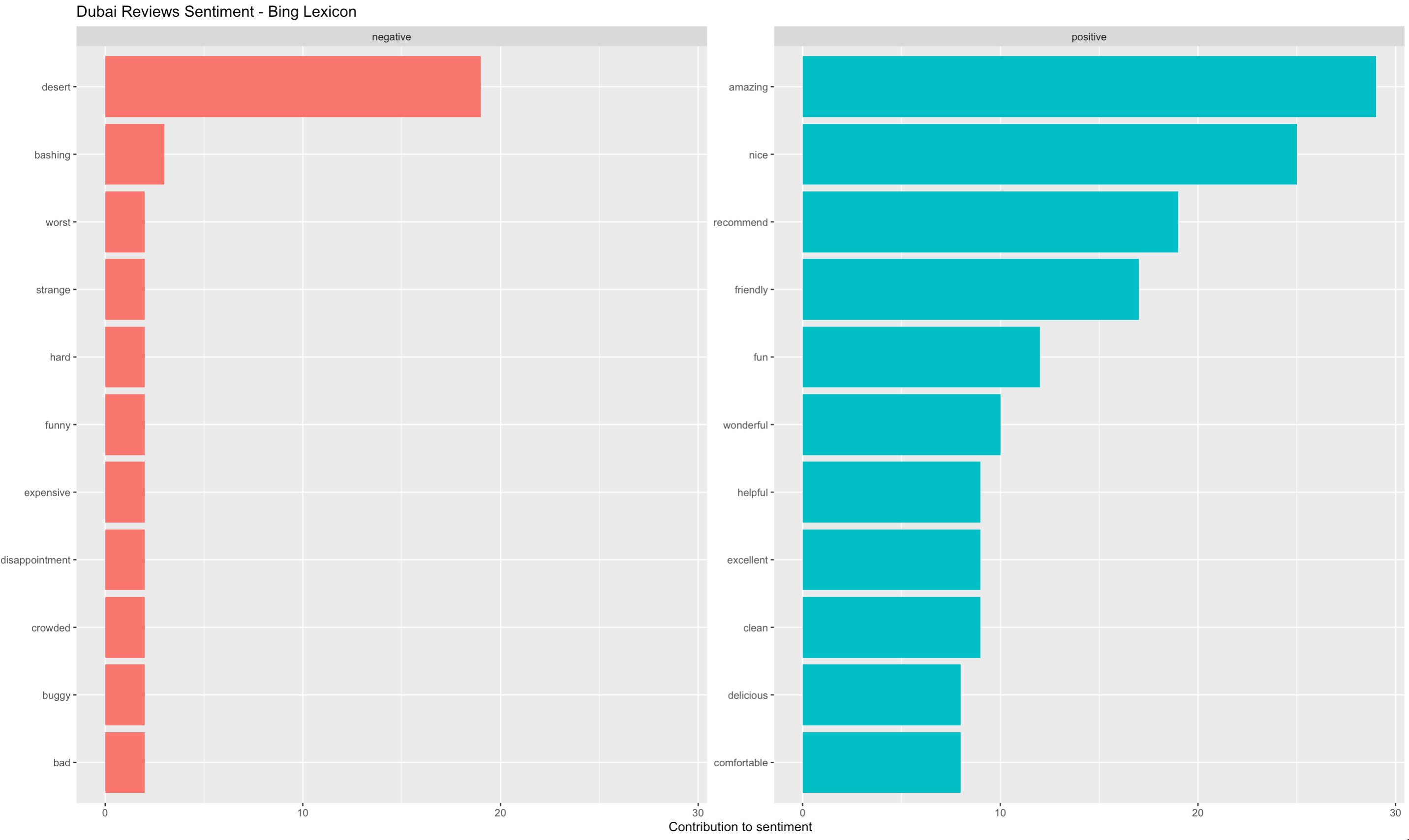
Note that the analysis was conducted using the Bing lexicon. This lexicon simply classifies words as positive or negative. In the case of Dubai, the lexicon classified the word “desert” as a negative word as it took it by the meaning of abandonment. In this case however, it means the type of land, a characteristic of the United Arab Emirates region.
Positive words used in all three cities include: “nice”, “amazing”, “recommend”, “friendly”, “clean”, “delicious”. However, Boston seems to a colder city (“cold” and “chilly” are amongst the most frequent words in reviews) and London is expensive, noisy and can be disappointing. Surprisingly, Dubai reviews frequently included words such as “bashing”, “worst” and “strange”. These suggest travelers should be cautious and prepared.
Differences between Boston, Dubai and London
In the sentiment analysis, both Dubai and London had frequently the word “expensive” in their reviews. This suggests that if a traveler is on a budget, they should consider Boston between these three options. But how and by how much is Boston different from Dubai and London?
It turns out that compared to Boston, both Dubai and London are very similar! The high positive correlation coefficients (0.77 and 0.74 respectively) show that reviews for London and Dubai are very similar to those for Dubai.
# STEP 4: Correlation coefficients

cor.test(data=frequency[frequency$city == "Dubai",],  ## very high 0.74
         ~proportion + `Boston`)

cor.test(data=frequency[frequency$city == "London",], ## very high 0.77
         ~proportion + `Boston`)
To take a closer look at what makes Dubai and London expensive for travelers, we can compute the proportion of each word within the total reviews and compare them with the Boston proportions:
# calculating proportions
frequency <- bind_rows(mutate(boston_tokens, city="Boston"),
                       mutate(dubai_tokens, city= "Dubai"),
                       mutate(london_tokens, city="London")
)%>%
  mutate(word=str_extract(word, "[a-z']+")) %>%
  count(city, word) %>%
  group_by(city) %>%
  mutate(proportion = n/sum(n))%>%
  select(-n) %>%
  spread(city, proportion) %>%
  gather(city, proportion, `Dubai`, `London`) %>%
  filter(proportion> 0.0001)

# plotting the correlogram
ggplot(frequency, aes(x=proportion, y=`Boston`,
                      color = abs(`Boston`- proportion)))+
  geom_abline(color="grey40", lty=2)+
  geom_jitter(alpha=.1, size=2.5, width=0.3, height=0.3)+
  geom_text(aes(label=word), check_overlap = TRUE, vjust=1.5) +
  scale_x_log10(labels = percent_format())+
  scale_y_log10(labels= percent_format())+
  scale_color_gradient(limits = c(0,0.001), low = "darkslategray4", high = "gray75")+
  facet_wrap(~city, ncol=2)+
  theme(legend.position = "none")+
  labs(y= "Boston", x=NULL)
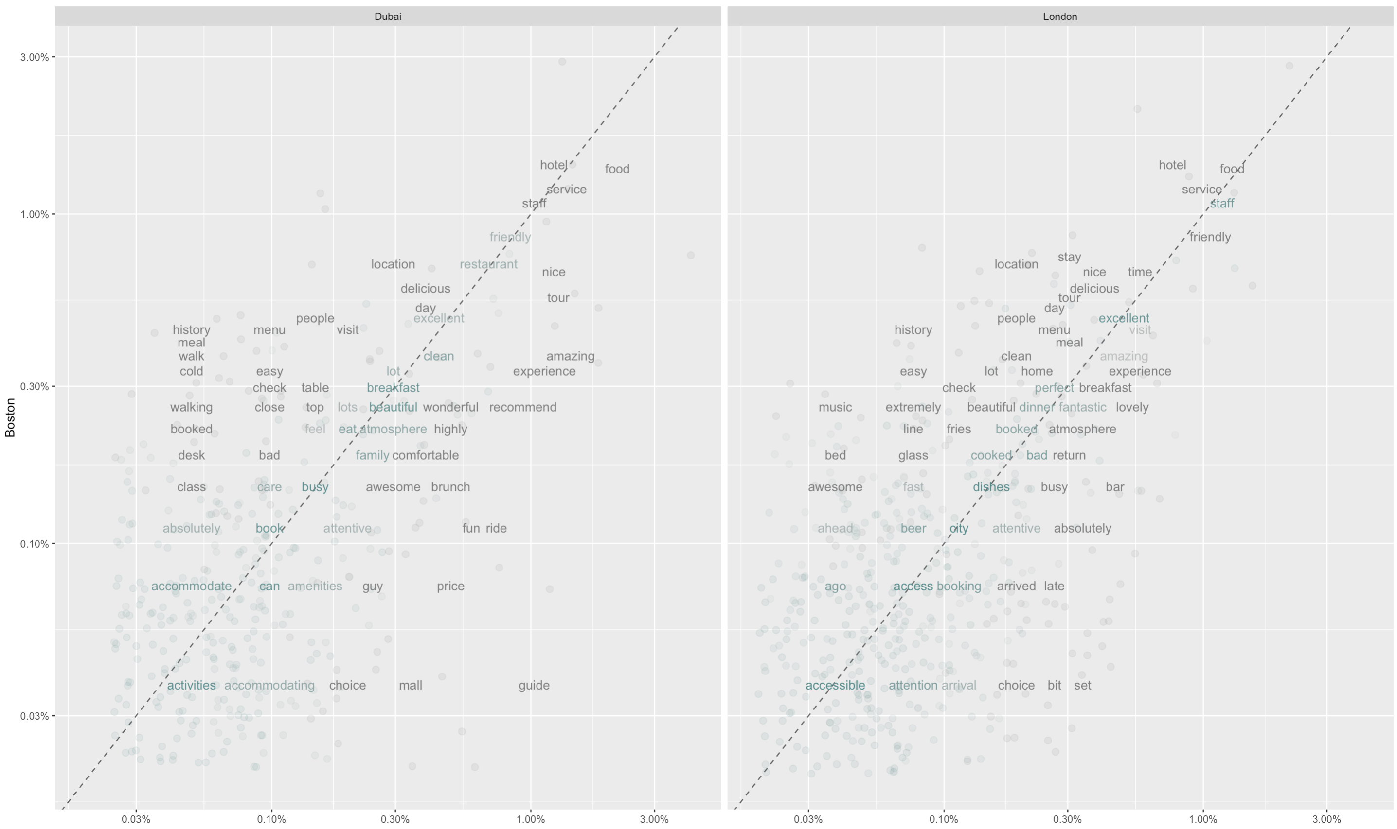
We can identify one group of words that are related to the travel industry: hotel, food, service and staff. These are most likely the objects being reviewed on TripAdvisor.com and explain the high correlation level.
Most interesting are words located in the left/upper corner and right/lower corner. On the left/upper corner are words that appear in the Boston reviews but not as frequent on Dubai and London reviews. It appears that Boston has more historical places and is walk-friendly. On the right/lower corner of each graph are words particular to London and Dubai. We see that London seems to be similar to Boston but has more nightlife with music sets and bars.
However, if one is interested in going to Dubai, one should look into guides, tours as the experiences people have reviewed were in that context.
Each Travel Experience is Unique
When choosing our next travel destination, we usually want an experience that is unique. Looking at reviews, we can identify certain key terms that are unique to each city’s experience. Here, instead of using individual words, the analysis is conducted on bigrams, or word couples since we want to have a better idea of the context in which these words were used.
# Merging tokens from all 3 cities
all_cities_df <- bind_rows(mutate(boston_tokens, city="Boston"),
                           mutate(dubai_tokens, city= "Dubai"),
                           mutate(london_tokens, city="London")
)

# Tokenizing bigrams, filtering out stop words, and counting frequencies
cities_bigrams <- all_cities_df %>%
  unnest_tokens(bigram, word, token = "ngrams", n=2) %>%
  separate(bigram, c("word1","word2"), sep = " ") %>%
  filter(!word1 %in% stop_words2$word) %>%
  filter(!word2 %in% stop_words2$word)  %>%
  count(city,word1, word2, sort=T) %>%
  ungroup()

# Grouping by city with sum of frequency
cities_bigrams2 <- cities_bigrams %>%
  group_by(city) %>%
  summarize(total=sum(n))

# Joining summed frequency to original bigrams dataset
cities_bigrams_leftjoined <- left_join(cities_bigrams, cities_bigrams2)

# Calculating TF-IDF for each
tidy_cities_bigrams_tfidf <- cities_bigrams_leftjoined %>%
  unite(bigram, word1, word2, sep=" ") %>%
  bind_tf_idf(bigram, city, n) %>%
  arrange(desc(tf_idf))

# Graphing TF-IDF
tf_idf_bigram_graph <- tidy_cities_bigrams_tfidf %>%
  arrange(desc(tf_idf)) %>%
  mutate(bigram=factor(bigram, levels=rev(unique(bigram)))) %>%
  group_by(city) %>%
  top_n(5,tf_idf) %>%
  ungroup %>%
  ggplot(aes(bigram, tf_idf, fill=city))+
  geom_col(show.legend=FALSE)+
  labs(x=NULL, y="tf-idf")+
  facet_wrap(~city, ncol=2, scales="free")+
  coord_flip()
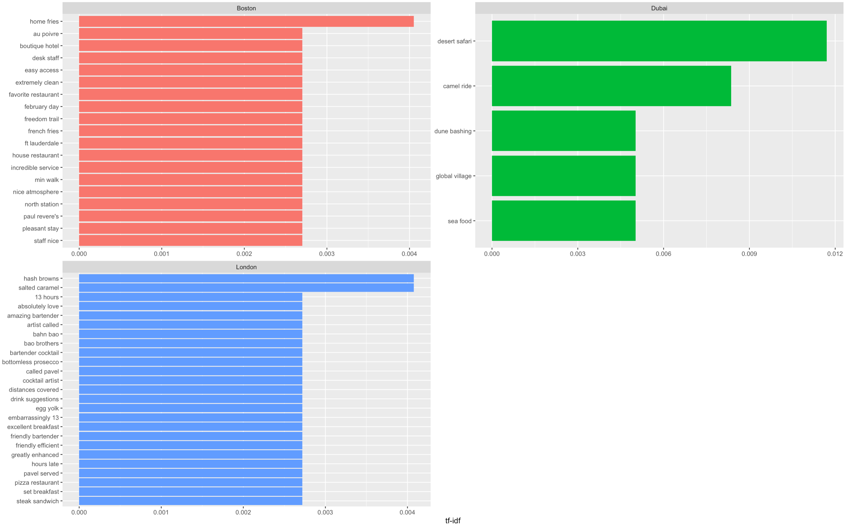
A note in the importance of context: the most important term in Dubai is “dune bashing”. Dune bashing is an off-road sport conducted in sand dunes. Previously in the sentiment analysis, we had seen “bashing” classified as a negative word due to its violent meaning, but when put into its context we now know reviewers were referring to the experience in Dubai and not safety!
The TF-IDF analysis helps us identify terms that are not the most frequent but are important in a collection of documents. The higher the TF-IDF of a word, the higher its importance, or uniqueness to that group of reviews.
Here, we can see that London contains multiple terms related to night life such as “amazing bartender”, “bottomless prosecco”, “cocktail artist”. This confirms our assumption in the correlogram above that London has nightlife as opposed to Boston. Dubai on the other hand includes mostly desert activities as well as “global village” - an attraction park. Therefore, party- goers might choose London whereas families might prefer Dubai’s experience.
Caveats
-
When analyzing social media reviews, we need to take into consideration that people who post reviews online, usually have a strong sentiment (either positive or negative) towards the object under evaluation (Beaton, 2018). For that reason, text analysis of such data should not be limited to sentiment analysis and should extend further into other techniques.
-
Another aspect of using user-based reviews are typos, which for the purpose of this analysis were not removed in data cleaning.
-
As this is a travel worldwide website, users from all over the world publish reviews in English. This leads to some differences in the English expressions used. For instance, “absolutely” was a frequent word in London reviews as it is more common in British English as opposed to Boston reviews.
-
For the purpose of this report, the Bing lexicon was used and classified the word “desert” as a negative word as it took it by the meaning of abandonment and not the characteristic of the land. However, for more accurate analysis, using a context/industry specific lexicon can improve the analysis accuracy and reduce mistakes in interpretability.
Conclusion
When choosing the next destination for travelling, we tend to get overwhelmed with reviews online on travel blogs. This report analyzed 100 reviews from Boston, Dubai and London on TripAdvisor.com.
The analysis used word sentiments, correlation graphs and bigrams word and document frequency to identify characteristics of each of the city. With this analysis, a traveler can be easily informed from reviews about each city’s price levels, food options and experience uniqueness. Then based on personal situation such as budget, travelling with family or friends and climate, one can make an informed decision as to where they would like to go.
A further application of this type of analysis could be used by TripAdvisor.com to summarize review pages for cities in real time. This would help users to sort through the most relevant reviews and make the process on the page more frictionless.