IBM: Predicting Employee Attrition

Note: This project was a collaboration with Ana Oliveira , Ivan Manurung and Nandish Hebbal in the context of a Data Mining class with Professor Thomas Kurnicki at Hult International Business School.

All the queries and analysis below were executed on Dataiku DSS.

The video and demo of the presentation described below can be found here. The original dataset and PySpark scripts can be found here (without the SQL cleaning steps).

Introduction

What is IBM?

International Business Machines Corporation (IBM) is an American multinational technology with operations in over 170 countries and founded in 1911. It produces and sells computer hardware, middleware and software, and provides hosting and consulting services, and is also a major research organization. It currently employs 352,600 people.

Dataset

Number of observations: 1470
Target Variable: Attrition = Employee leaving the company (0 = no, 1 = yes)
Business Case: Retention = Employee staying in the company

Our focus: Enabling IBM to reduce attrition

Why?

• Low retention leads to high costs, such as the cost of disruption, onboarding and training of new hires;
• These costs can be reduced by implementing attrition prevention policies and allocating HR resources more accurately

Key Questions:

• What is the probability of an employee leaving the company?
• What are the key indicators/drivers of an employee leaving the company?
• What actionable insights can result in a revised Retention Strategy to improve employee retention?

How?

1. Data exploring & cleaning: Identifying and understanding the drivers of employee attrition;
2. Using classification models to predict the individual attrition risk of employees;
3. Implementing a score model

Methodology, Exploratory Data Analysis & Limitations

Methodology

1. One-hot encoding categorical variables (SQL)
2. Data Cleaning Through Flags (SQL)
3. Correlation Matrix (Pandas)
4. Base Model with Logistic Regression (PySpark)
5. Machine Learning Models to determine important features (Dataiku)
6. Building a Weighted Scoring Model, using a new logistic regression as a basis for weights (SQL and PySPark);
7. Confusion Matrix (Dataiku)

Exploratory Data Analysis

• The strongest positive correlations with the target features are:
  • Overtime (0.25)
  • Business Travel (0.13)
• The strongest negative correlations with the target features are:
  • Job Level (-0.17)
  • Age (-0.16)
  • Years in Current Role (-0.16)
  • Monthly Income (-0.16)
• Single employees show the largest proportion of leaving employees
• Employees living further from work are more likely to leave
• Employees traveling frequently are more likely to leave
• Employees working overtime are more likely to leave
• Employees with higher # of previous companies are more likely to leave

Limitations

It should be disclaimed that the model should not be used to shape hiring policies as it takes variables into consideration (such as age and gender) which could lead to discriminatory and illegal HR recruiting practices;

Attrition seems to encompass cases when people left voluntarily but also people that were fired, retired etc. For best results, we would have to have access to data that broke down attrition so that we could identify only cases when people quit.

Additional Limitations:

• Total Years was probably not logged properly (Years at company = Total Years Working for adults older than 45)
• Years at company and promotions and current roles do not match (Data collection problem)
• There’s no quantitative data on over time, it’s just a true or false
• Job level - assumption that a higher value means higher job level. People with higher job levels are more likely to retire, therefore this might influence this variable and it’s correlation.

Model Development

Data Cleaning in SQL

To ensure a proper functioning of the classification models, we first translated the target variable into a boolean with 1 and 0:

SELECT *,
CASE 
    WHEN "Attrition" = True THEN 1 
    ELSE 0
END AS boolean_attrition
FROM "TEAM12IBM_ibm__original_sql";

We did the same to other categorical variables, such as business travel:

SELECT *,
CASE 
    WHEN "BusinessTravel" = 'Travel_Rarely'       THEN 1
    WHEN "BusinessTravel" = 'Travel_Frequently'   THEN 2  
    WHEN "BusinessTravel" = 'Non-Travel'          THEN 0  
    
    ELSE 0
END AS boolean_businesstravel
FROM "TEAM12IBM_ibm_clean";

This method allowed us to group certain categorical variables into similar groups, in order to increase our model’s applicability across the company:

SELECT *,
CASE 
    WHEN "JobRole" = 'Sales Representative' OR 
         "JobRole" = 'Manager' OR 
         "JobRole" = 'Human Resources' OR 
         "JobRole" = 'Sales Executive'
         THEN 0
    WHEN "JobRole" = 'Research Director' OR
         "JobRole" = 'Laboratory Technician' OR
         "JobRole" = 'Research Scientist' OR
         "JobRole" = 'Healthcare Representative' OR
         "JobRole" = 'Manufacturing Director'
         THEN 1  
    ELSE 999
END AS boolean_JobRole
FROM "TEAM12IBM_ibm_clean";

Note: here, we included an ELSE clause with “999”. This will ensure that if there is a data entry typo or if we forgot a category in the query, it will be flagged easily for retrieval.

During our exploratory data analysis, we found certain inconsitencies which needed to be flagged. For instance, certain employees had equal “Years At Company” and “Total Working Years” even though they were older than 45. The flagging will help us in case we decide to remove these observations from our dataset.

-- Flagging the inconsistencies
SELECT *,
CASE 
    WHEN "YearsAtCompany" = "TotalWorkingYears" AND "Age" > 45 THEN 1 
    ELSE 0 
    END AS "TotalWorkingYears_flag"
FROM "TEAM12IBM_ibm_clean";

-- Filterting the observations out
SELECT *
FROM "TEAM12IBM_ibm_clean"
WHERE "TotalWorkingYears_flag" = 0;

Model Selection

Step 1: Correlation Matrix (Python - pandas)

corr_matrix = df_pd.corr()
corr_matrix['boolean_attrition'].sort_values()

Using the strongest correlations (both negative and positive), we then build a base line Logistic Regression model. The goal is to compare the results of any other models to this one, to evaluate if the prediction power increases with the level of model complexity.

Step 2: Base Line Logistic Regression (PySpark)

Set-up:

%pylab inline

# Importing dataframe essential packages
import dataiku
from   dataiku import pandasutils as pdu
import pandas as pd

# Importing PySpark Packages
import dataiku.spark as dkuspark
import pyspark
from pyspark import SparkContext, SparkConf
from pyspark.sql import SQLContext
from pyspark.ml import Pipeline
from pyspark.ml.classification import LogisticRegression
from pyspark.ml.feature import HashingTF, Tokenizer, CountVectorizer
from pyspark.sql import Row
from pyspark.sql.functions import UserDefinedFunction
from pyspark.sql.types import *
from pyspark.ml.feature import VectorAssembler
from pyspark.mllib.evaluation import *
from pyspark.ml.evaluation import BinaryClassificationEvaluator
from pyspark.ml.tuning import ParamGridBuilder, CrossValidator

# Load PySpark
sc = pyspark.SparkContext.getOrCreate()
sqlContext = SQLContext(sc)

Since we’re using the dataset cleaned within Dataiku, we run the following lines to read the dataset with dataiku then as Pandas and Spark:

# Read Dataiku dataset from memory
mydataset = dataiku.Dataset("IBM_clean_Hadoop")

# Read the dataset as a Pandas Dataframe
df_pd = mydataset.get_dataframe()

# Read the dataset as a Spark dataframe
df_sprk = dkuspark.get_dataframe(sqlContext, mydataset)

We’ll want to check if our dataframe is cleaned. Since we have removed some observations, our dataset should have 1447 rows, and additional features we engineered with SQL.

# Get the count of records in the dataframe
print(df_sprk.count())

# Get a view of the first 5 records in the dataframe
df_pd.head()

1447

After checking the dataset, we can start building our base model:

# creating vectors with variable names
x_var_vec = VectorAssembler(inputCols = ['boolean_overtime',
                                         'boolean_businesstravel',
                                         'Age',
                                         'YearsInCurrentRole',
                                         'MonthlyIncome',
                                         'StockOptionLevel',
                                         'JobSatisfaction',
                                         'NumCompaniesWorked',
                                         'JobInvolvement'], outputCol = "features")

# Adding x var vector back into dataframe
vec_to_df = x_var_vec.transform(df_sprk)

# Defining target variable
df_logit = vec_to_df.select(['features', 'boolean_attrition']) 

# Renaming Target Column
df_logit = df_logit.withColumnRenamed("boolean_attrition", "label")

# Splitting the dataset
splits = df_logit.randomSplit([0.7,0.3])
train_df = splits[0]
test_df = splits[1]

# Creating an object with Logistic Regression Model
lr       = LogisticRegression(maxIter = 20)
pipeline = Pipeline(stages = [lr])

# fitting the model 
model = lr.fit(train_df)

# Calculating Evaluation Metrics
result    = model.transform(test_df)
evaluator = BinaryClassificationEvaluator(rawPredictionCol = "rawPrediction")
AUC_ROC   = evaluator.evaluate(result,{evaluator.metricName: "areaUnderROC"})
coefs     = model.coefficients
intercept = model.intercept

We’ll also run a Parameter GridSearch and CrossValidation. These will help improve our model’s predictive capabilities.

## Setting up Parameter GridSearch and CrossValidation
# Create ParamGrid for Cross Validation
paramGrid = (ParamGridBuilder()
             .addGrid(lr.regParam, [0.01, 0.5, 2.0])
             .addGrid(lr.elasticNetParam, [0.0, 0.5, 1.0])
             .addGrid(lr.maxIter, [1, 5, 10])
             .build())
# Create 5-fold CrossValidator
cv = CrossValidator(estimator=lr, estimatorParamMaps=paramGrid, evaluator=evaluator, numFolds=5)

# Run cross validation
cvModel = cv.fit(train_df)

# Calculating Evaluation Metrics
result_cv    = cvModel.transform(test_df)
evaluator_cv = BinaryClassificationEvaluator(rawPredictionCol = "rawPrediction")
AUC_ROC_cv   = evaluator_cv.evaluate(result_cv,{evaluator_cv.metricName: "areaUnderROC"})
coefs_cv     = cvModel.bestModel.coefficients
intercept_cv = cvModel.bestModel.intercept

print('LOGISTIC REGRESSION: After CV')
print('AUC ROC:' + str(AUC_ROC_cv))
print('Coefficients:' +  str(coefs_cv))
print('Intercept:' + str(intercept_cv))

LOGISTIC REGRESSION: After CV
AUC ROC: 0.820729684909
Coefficients: [0.35658374691111, 0.13735670630940452, -0.00977140480720, -0.018882556136572, -1.50013019973230, -0.09564407673339921, -0.0626493550002785551, 0.015438513313969211, -0.1082495785327109]
Intercept: -0.95818648954566542 

The most important number in these results is the AUC ROC score (area under the curve). This number represents our model’s predictve capabilities. A score of 0.82 is not bad at all! The coefficients in a logistic regression need to be treated differently than with linear regressions. We first need to take the exponential of a coefficient, which represents the change in odds ratio. For example, for every additional companie worked at in the past, an employees odds of leaving IBM increase by exp(0.015)-1)*100 = 1.56 %.

With this base model, we can then compare different models using Dataiku’s Visual Analysis tools.

Step 2: Model Competition

Using all relevant variables, and the same level of data splitting, we conducted an analysis with 6 different models:

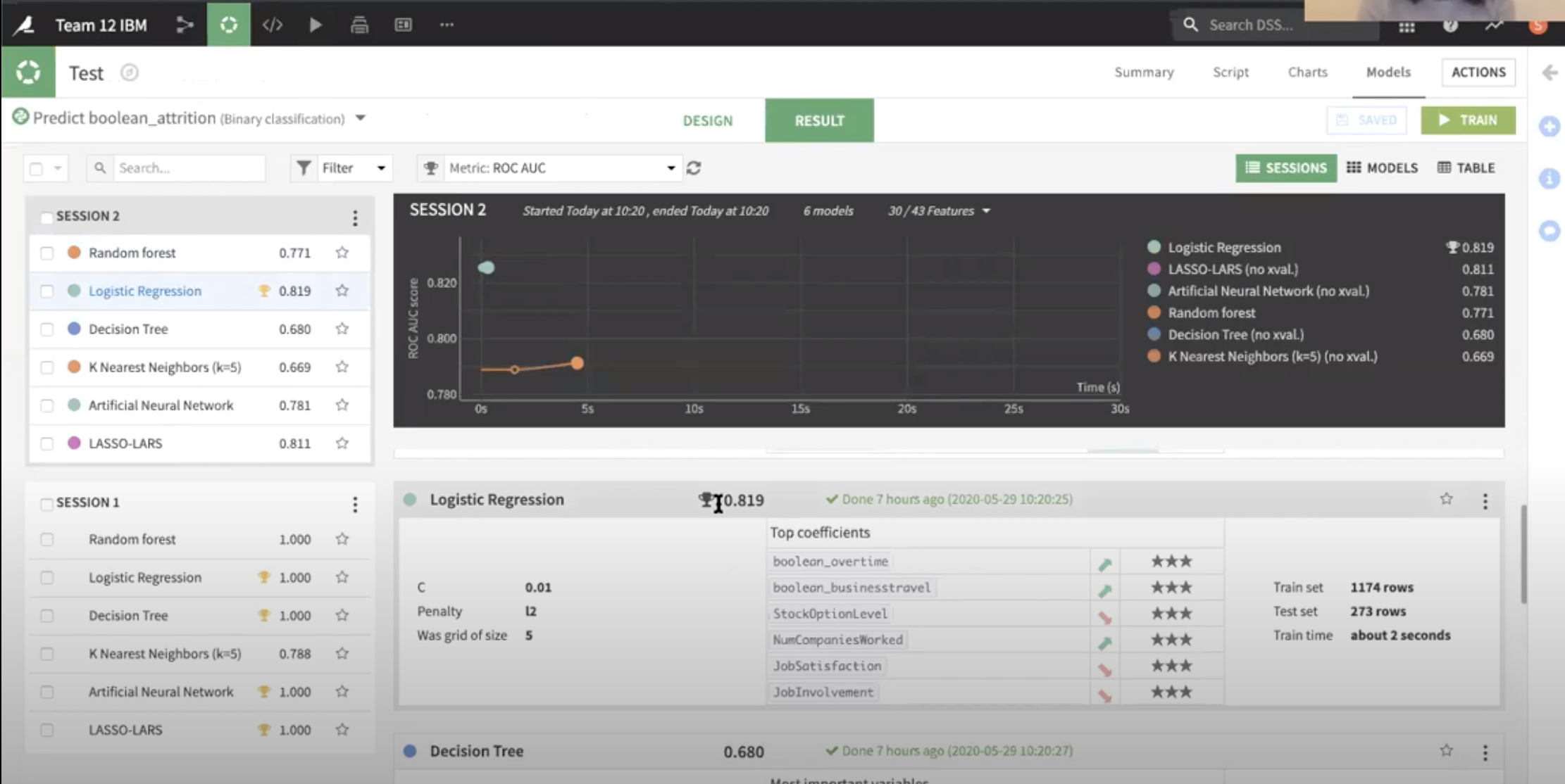
As you can see, the lab concluded that a logistic regression yields the best predictive power, even against different andvanced and complex models.

The variables with the most significant power are slightly different from our previous results. Previously we had:

• boolean_overtime
• boolean_businesstravel
• Age
• YearsInCurrentRole
• MonthlyIncome
• StockOptionLevel
• JobSatisfaction
• NumCompaniesWorked
• JobInvolvement

Now:

• boolean_overtime
• boolean_businesstravel
• StockOptionLevel
• NumCompaniesWorked
• JobInvolvement

The AUC ROC score has also slighlty decreased. However, the second model has a lot more value for the case. By using less features, and still yielding a extremely powerful score, we are able to prioritize business resources to these 5 variables, and achieve a similar outcome!

Model Precision & Main Findings

Confusion Matrix (Logistic Regression) on Total Test Observations

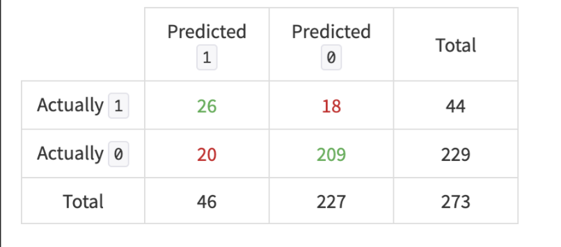
The confusion matrix above shows how our model tested against the test data. Where 1 is the case of an employee leaving the company and 0 of the employee staying we can see that our model correctly predicted the outcome on 86% of the cases. Our model is also capable to predict 60% of all employees that left. With this model, HR efforts can be allocated more efficiently to increase retention rates.

• Stock Option Level, Job Satisfaction and Job Involvement increase the probability of retention of employees
• Overtime, Business Travel and Number of Companies Worked increase the probability of employees leaving

Business Insights & Recommendations

• A Retention Strategy can be design for each of the three Risk Score groups.

• In person interviews with employees led by HR, with a focus on medium and high-risk employees can provide further insight .

• When Attrition could not be preventing, establishing “exit interviews” could be an additional tool to gather honest insight.

Overtime

• Efforts must be taken to appropriately gauge human resource needs and allocation to reduce overtime needs;
• Adequate support should be offered to employees who frequently engage in overtime;
• Percent increases in individual employee’s overtime should be flagged and best practices put in place;
• Collect more detailed data as a continuous variables as opposed to binary

Business Travel

• Divide traveling needs equitably by employees;

• Identify employees who have a personal preference for business travelling;

• Adjust travel frequency of employees flagged as “high-risk”;

Job Involvement & Satisfaction Score

• Team building activities increase social connection and therefore job involvement;

• Conduct individual interviews if there is a decrease in job involvement for a specific group of employees;

Stock Options Level Score

• For future business insights, collect data on length of vesting period to calculate correlation with attrition;

• Revise compensation structure if necessary to incentivize employee retention.